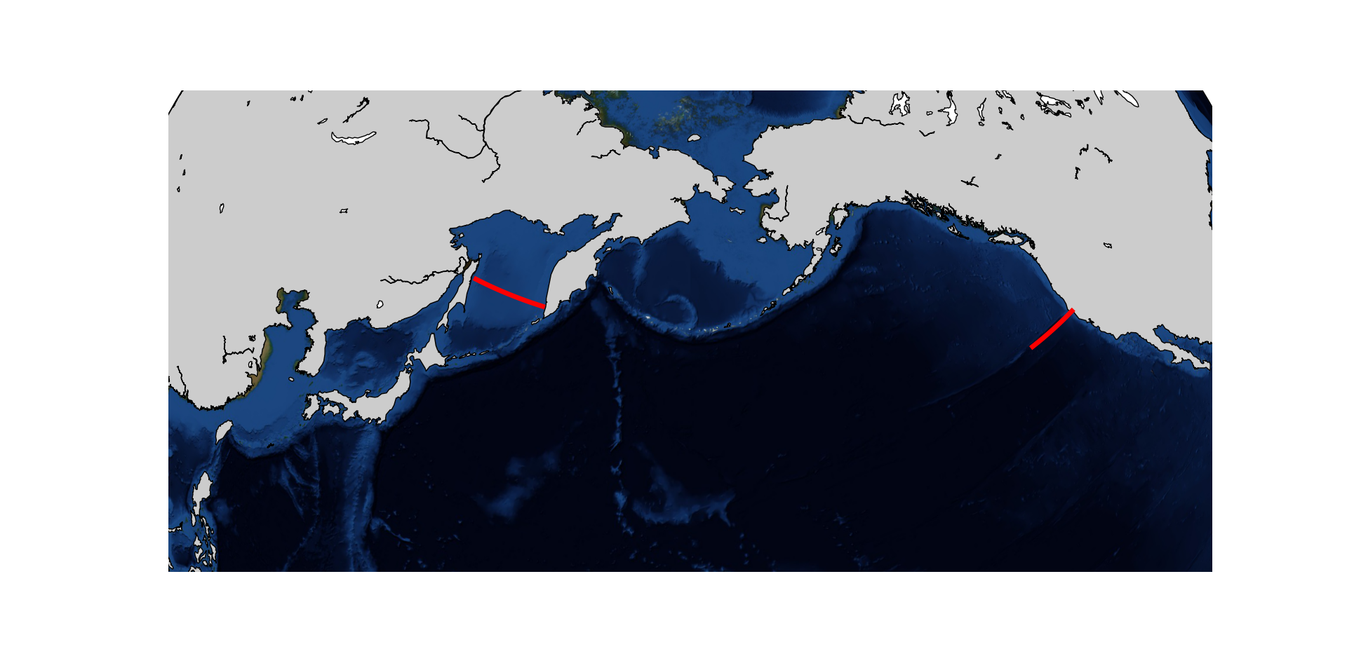
The regions selected for comparison between CESM2+CICE and CESM2+DICE.
This was a project during a GCM (Global Climate Modeling) class at the Geography department that Dr. Kooperman lectured. For my project I wanted to see how the dense shelf water (DSW) from the sea of Okhotsk would affect the DO dynamics in the CCS.
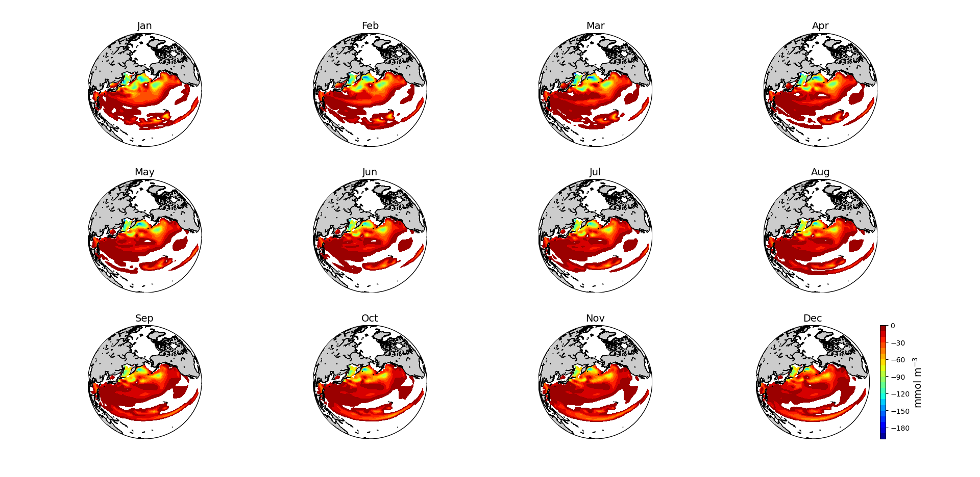
CESM 2 was used in order to understand the indirect feedback of the sea ice in the CCS. CESM2 is a coupled model that has atmosphere, land, land ice, river runoff, ocean, sea ice, and wave components. Two simulations were done, one with an active sea ice model (CICE) and the other one with a dataset (DICE SSMI). The simulation using DICE SSMI was set to false to couple with the ocean model (POP) so it ran as a prognostic model. The length of the simulations were 1 year each with monthly output. Outputs were converted from curvilinear to lon lat using Climate Data Operator (CDO) version 1.9.9, data analysis was done using Python 3.6. The region of study was from 0-70°N and 100°W-250°W.
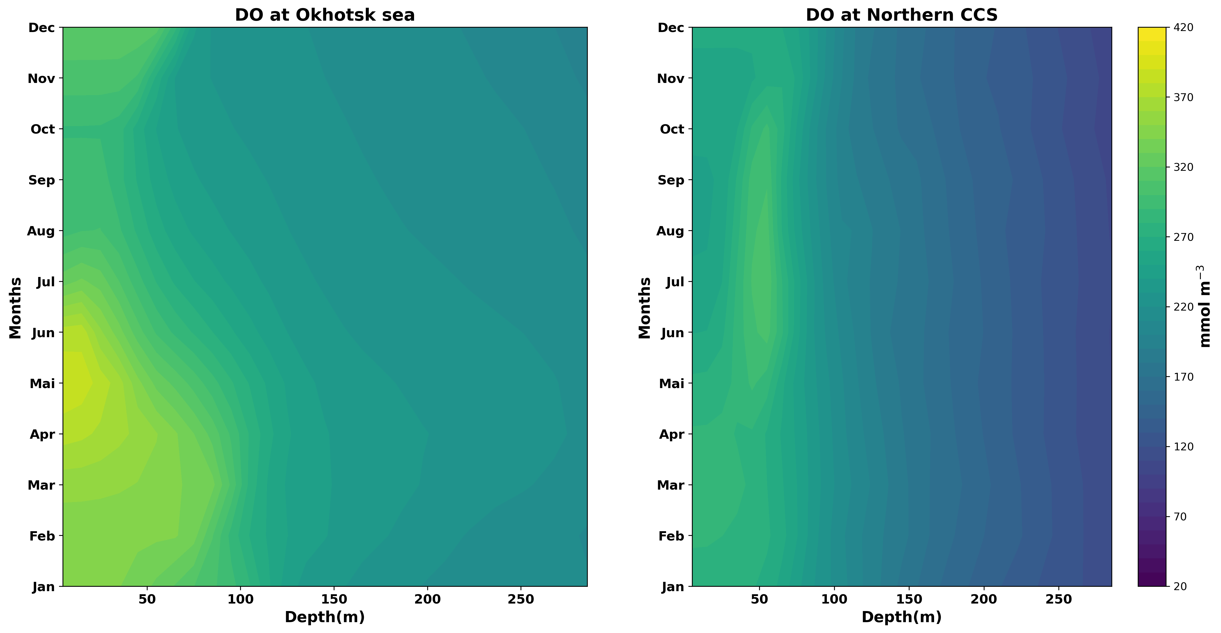
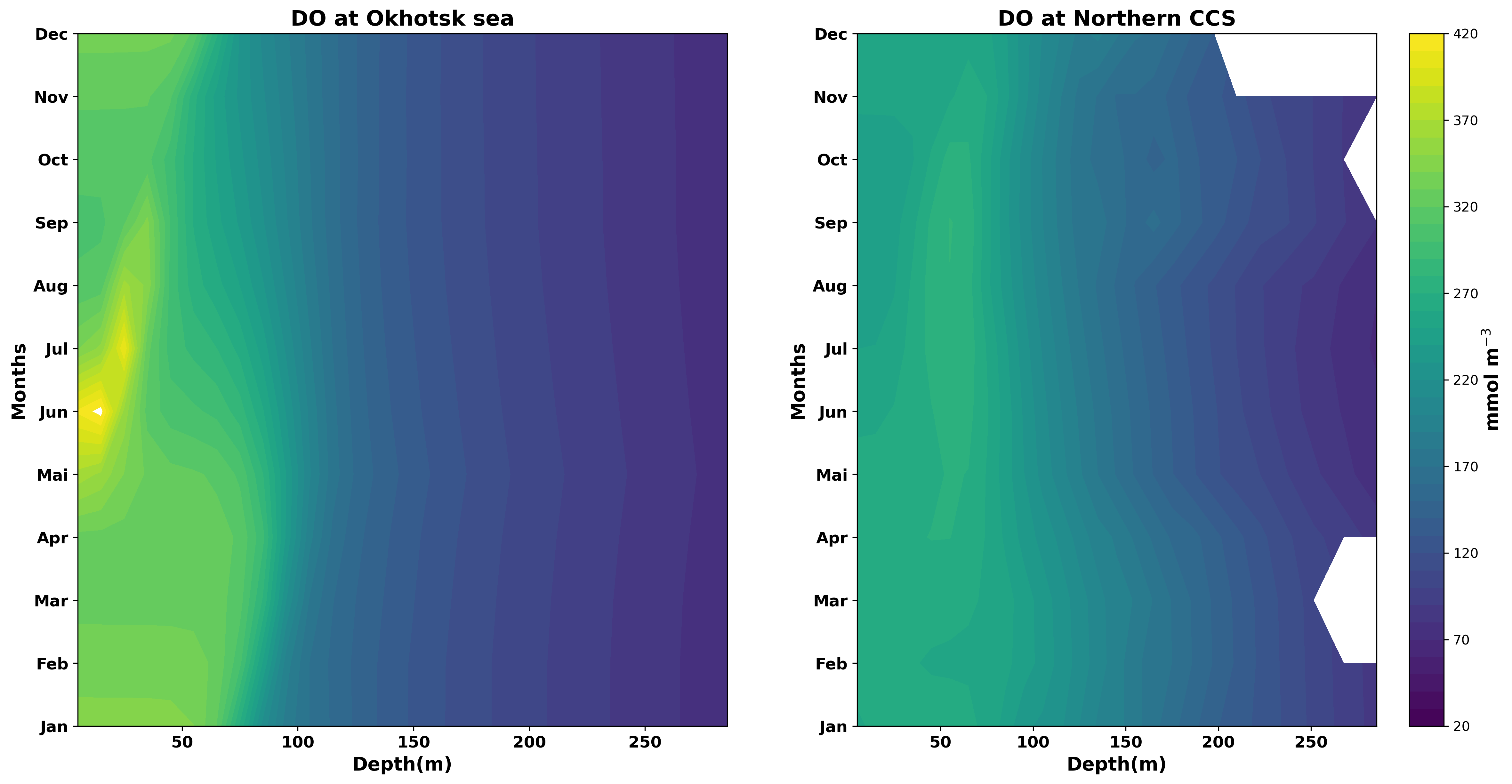
In an effort to separate the Dissolved Oxygen (DO) coming from the Subarctic current from the Undercurrent in the CCS, I decided to use negative velocities as my flag in the first 300 meters and within 700km from the coastline on the west coast of the US. Dissolved Oxygen at 150 meters were compared between the two simulations for the entire region.
To sum up, coupling an active sea ice model to POP affects the production of DO in the Okthotsk sea, and as a result, it will affect the DO being input in the CCS through the Subarctic current. There are changes in the timing and spread of maximum DO in the Okthotsk sea between the simulation with ice and without ice interaction. Less oxygenated waters are observed when coupling CICE with POP, and therefore, when there is no ice affecting the ocean processes the waters are more oxygenated.